Math worksheets grade 1
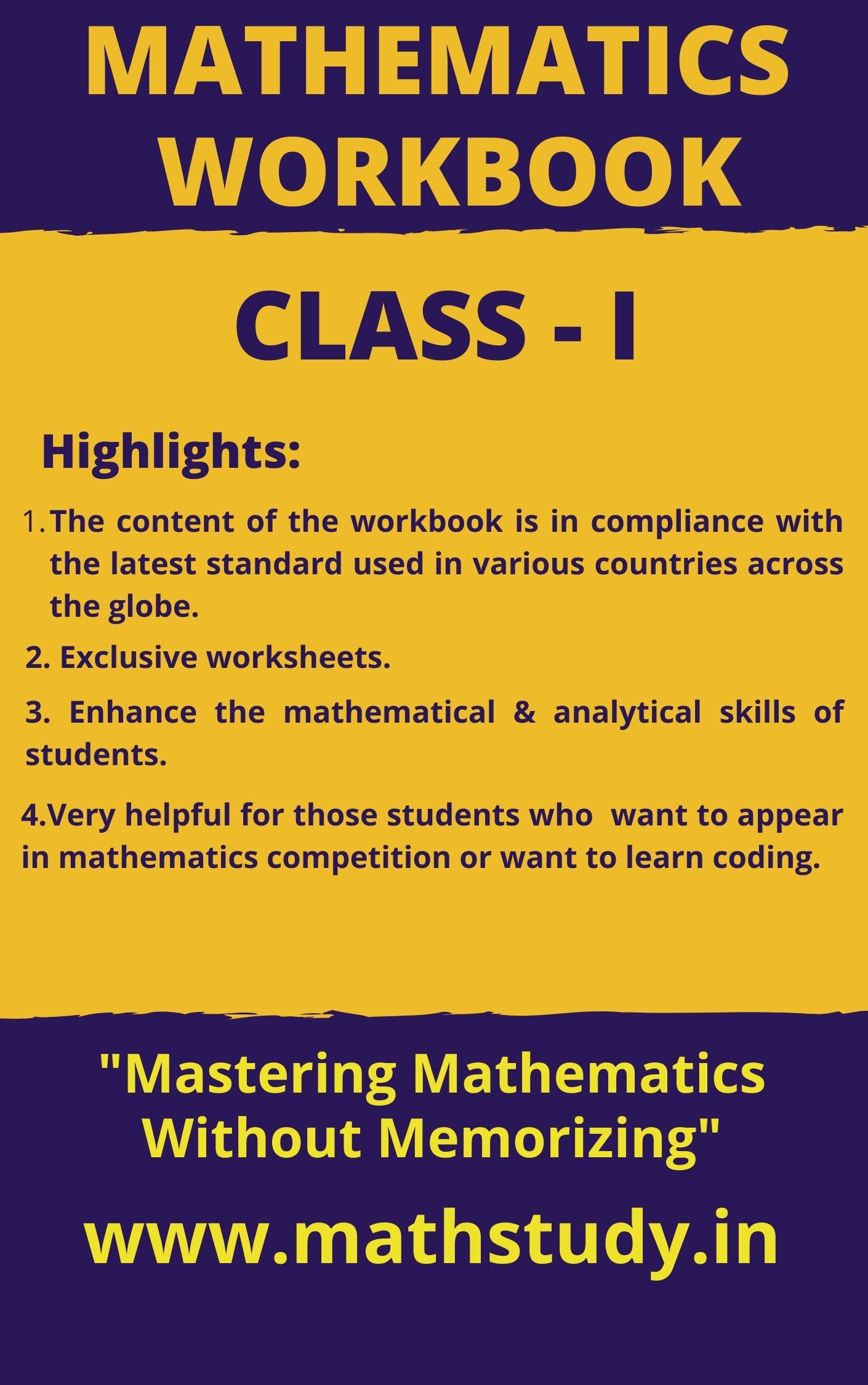
Math worksheets grade 1 Who can use this workbook? This workbook is useful for students of class 1 which is…
Math worksheets grade 1 Who can use this workbook? This workbook is useful for students of class 1 which is…
mathematics worksheet class 1 Who can use this workbook? This workbook is useful for students of class 1 which is…
Class 1 worksheets math Who can use this workbook? This workbook is useful for students of class 1 which is…
Best Math Workbook For 1st Grade-Printable Worksheets Who can use this workbook? This workbook is useful for students of class…
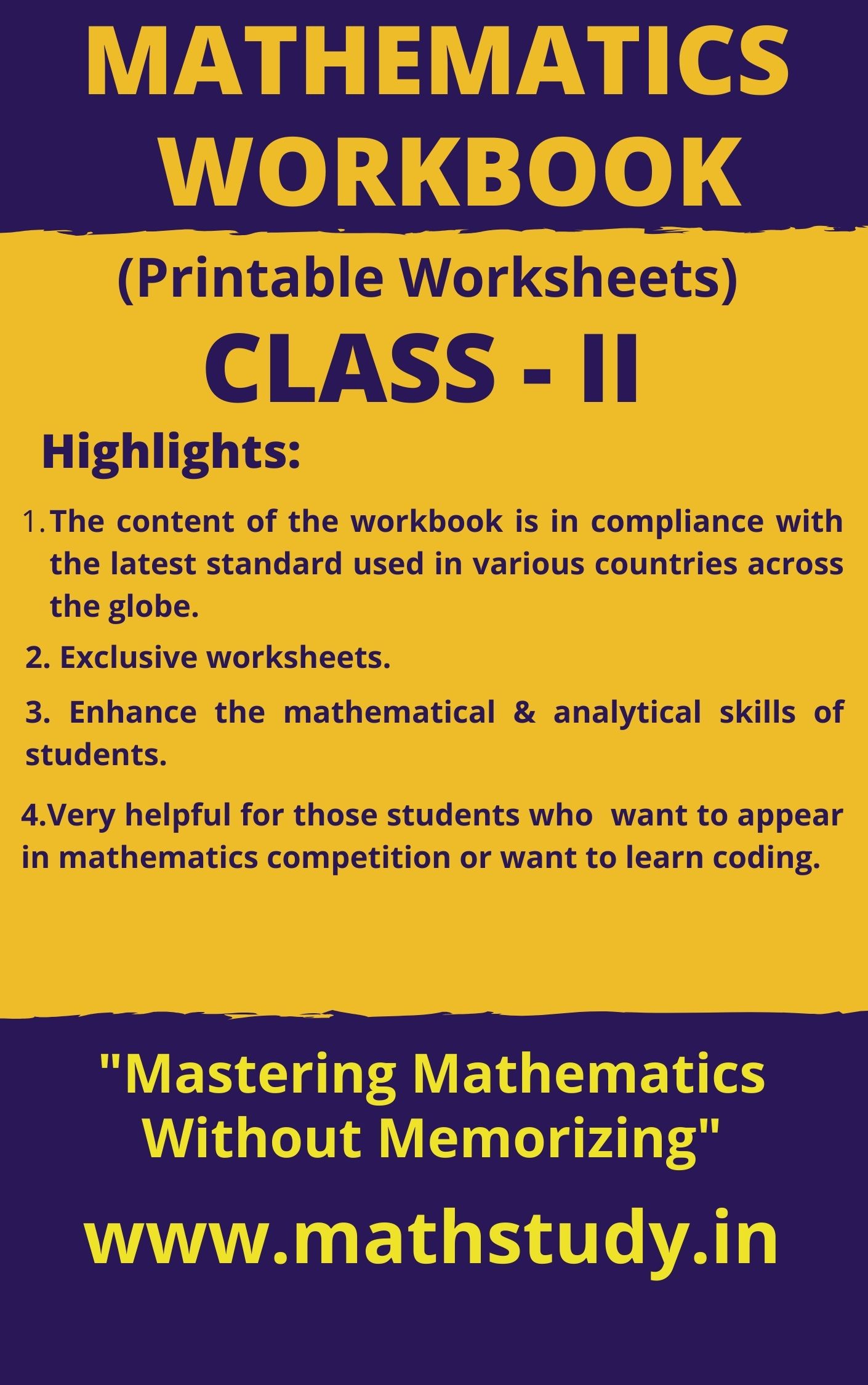
MATHEMATICS WORKBOOK CLASS – II ( Printable Worksheets) Who can use this workbook? This workbook is useful for students of…
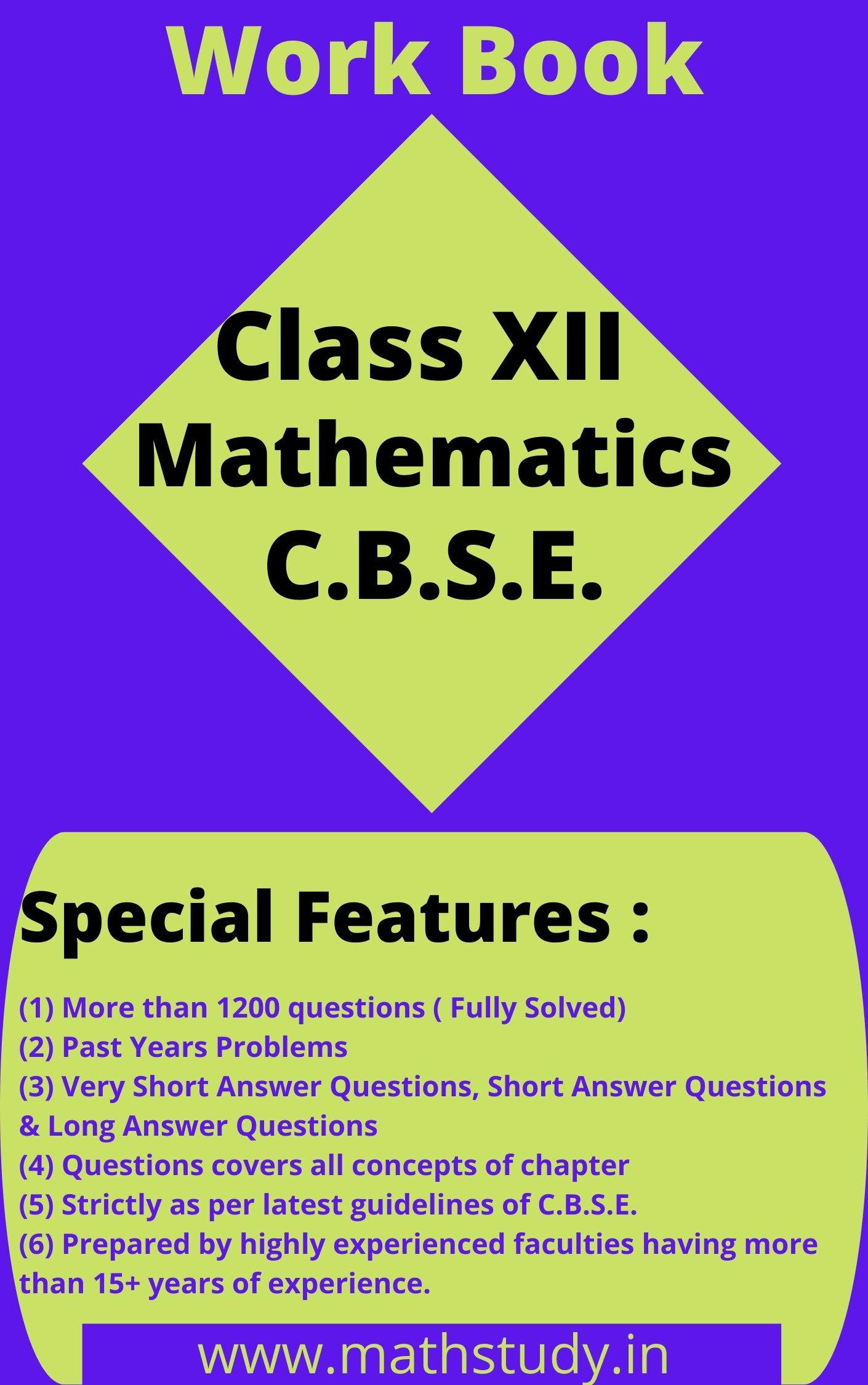
Class 12 math workbook fully solved C.B.S.E. Mathematics workbook class 12 Special Features : (1) More than 1200 questions (…
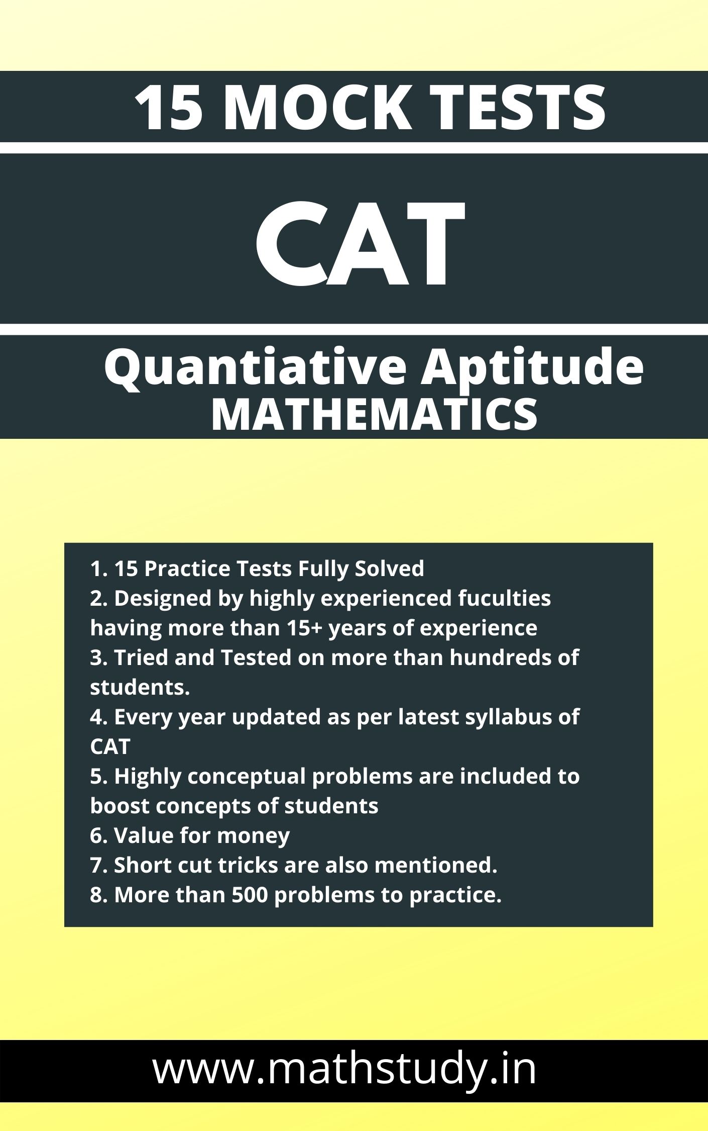
In this blog we are discussing few important points about CAT exam which will be very helpful for CAT aspirants…
Best Math Workbook For 1st Grade-Printable Worksheets BUY NOW 1. More than 150 worksheets. 2. Worksheets on word problems that…
Math Formula Book for JEE BITSAT Math Formula Book for JEE BITSAT Highly useful for class 11 & 12 students…

Class 12 Mathematics NCERT Solutions During the past 15 years our faculties have developed lot of study material for students…